相关概念
- Clustering: the process of grouping a set of objects into classes of similar objects
- high intra-class similarity
- low inter-class similarity
- the commonest form of unsupervised learning
- Unsupervised learning
- learning from raw (unlabeled, unannotated, etc) data, as opposed to supervised data where a classification of examples is given
Distance Measures

- Minkowski metric
$$ d(x, y)=\sqrt[r]{\sum_{i=1}^{p}\left|x_{i}-y_{i}\right|^{r}} $$
- Euclidean distance($r=2$)
$$ d(x, y)=\sqrt[2]{\sum_{i=1}^{p}\left|x_{i}-y_{i}\right|^{2}} $$
- Manhattan distance($r=1$)
$$ d(x, y)=\sum_{i=1}^{p}\left|x_{i}-y_{i}\right| $$
- Chebyshev distance($r=+\infty$)
$$ d(x, y)=\max _{1 \leq i \leq p}\left|x_{i}-y_{i}\right| $$
- Hamming distance
Manhattan distance is called Hamming distance when all features are binary.
- Pearson correlation coefficient
$$ s(x, y)=\frac{\sum_{i=1}^{p}\left(x_{i}-\bar{x}\right)\left(y_{i}-\bar{y}\right)}{\sqrt{\sum_{i=1}^{p}\left(x_{i}-\bar{x}\right)^{2} \times \sum_{i=1}^{p}\left(y_{i}-\bar{y}\right)^{2}}} $$ $$ \text { where } \bar{x}=\frac{1}{p} \sum_{i=1}^{p} x_{i} \text { and } \bar{y}=\frac{1}{p} \sum_{i=1}^{p} y_{i} $$
- cosine distance(Special case)
$$ s(x, y)=\frac{\vec{x} \cdot \vec{y}}{|\vec{x}| \cdot|\vec{y}|} $$
- Edit Distance
To measure the similarity between two objects, transform one of the objects into the other, and measure how much effort it took. The measure of effort becomes the distance measure.
K-Means
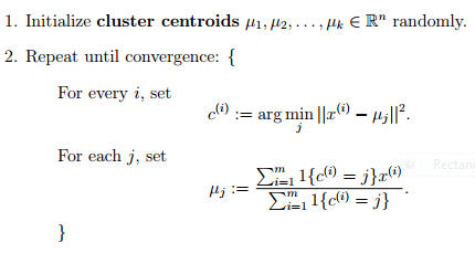
- 随机选取k个聚类质心点(cluster centroids)
- 重复下面过程直到收敛
- 对于每一个样例 i ,计算其应该属于的类
- 对于每一个类 j ,重新计算该类的质心
- simple implementation of kmeans here to just illustrate some concepts
import numpy as np
from numpy.linalg import norm


class Kmeans:
    '''Implementing Kmeans algorithm.'''

    def __init__(self, n_clusters, max_iter=100, random_state=123):
        self.n_clusters = n_clusters
        self.max_iter = max_iter
        self.random_state = random_state

    def initializ_centroids(self, X):
        np.random.RandomState(self.random_state)
        random_idx = np.random.permutation(X.shape[0])
        centroids = X[random_idx[:self.n_clusters]]
        return centroids

    def compute_centroids(self, X, labels):
        centroids = np.zeros((self.n_clusters, X.shape[1]))
        for k in range(self.n_clusters):
            centroids[k, :] = np.mean(X[labels == k, :], axis=0)
        return centroids

    def compute_distance(self, X, centroids):
        distance = np.zeros((X.shape[0], self.n_clusters))
        for k in range(self.n_clusters):
            row_norm = norm(X - centroids[k, :], axis=1)
            distance[:, k] = np.square(row_norm)
        return distance

    def find_closest_cluster(self, distance):
        return np.argmin(distance, axis=1)

    def compute_sse(self, X, labels, centroids):
        distance = np.zeros(X.shape[0])
        for k in range(self.n_clusters):
            distance[labels == k] = norm(X[labels == k] - centroids[k], axis=1)
        return np.sum(np.square(distance))

    def fit(self, X):
        self.centroids = self.initializ_centroids(X)
        for i in range(self.max_iter):
            old_centroids = self.centroids
            distance = self.compute_distance(X, old_centroids)
            self.labels = self.find_closest_cluster(distance)
            self.centroids = self.compute_centroids(X, self.labels)
            if np.all(old_centroids == self.centroids):
                break
        self.error = self.compute_sse(X, self.labels, self.centroids)

    def predict(self, X):
        distance = self.compute_distance(X, old_centroids)
        return self.find_closest_cluster(distance)
- Issues with Kmeans:
- K-means often doesn’t work when clusters are not round shaped because of it uses some kind of distance function and distance is measured from cluster center.
- Another major problem with K-Means clustering is that Data point is deterministically assigned to one and only one cluster, but in reality there may be overlapping between the cluster for example picture shown below
Gaussian Mixture Models(GMM)
-
In practice, each cluster can be mathematically represented by a parametric distribution, like a Gaussian (continuous) or a Poisson (discrete). The entire data set is therefore modelled by a mixture of these distributions. An individual distribution used to model a specific cluster is often referred to as a component distribution.
-
In this approach we describe each cluster by its centroid (mean), covariance , and the size of the cluster(Weight).
- 相对于k均值聚类算法使用 k 个原型向量来表达聚类结构,高斯混合聚类使用 k 个高斯概率密度函数混合来表达聚类结构
$$ P(x_{i}|y_{k}) = \frac{1}{\sqrt{2\pi\sigma_{y_{k}}^{2}}}exp( -\frac{(x_{i}-\mu_{y_{k}})^2} {2\sigma_{y_{k}}^{2}}) $$
- 于是迭代更新 k 个簇原型向量的工作转换为了迭代更新 k 个高斯概率密度函数的任务。每个高斯概率密度函数代表一个簇,当一个新的样本进来时,我们可以通过这 k 的函数的值来为新样本分类
高斯混合模型聚类算法EM步骤如下:

1. 猜测有几个类别,既有几个高斯分布。
2. 针对每一个高斯分布,随机给其均值和方差进行赋值。
3. 针对每一个样本,计算其在各个高斯分布下的概率。
4. 针对每一个高斯分布,每一个样本对该高斯分布的贡献可以由其下的概率表示,如概率大则表示贡献大,反之亦然。这样把样本对该高斯分布的贡献作为权重来计算加权的均值和方差。之后替代其原本的均值和方差。
5. 重复3~4直到每一个高斯分布的均值和方差收敛。
Hierarchical Clustering
1. Compute the proximity matrix
2. Let each data point be a cluster
3. Repeat: Merge the two closest clusters and update the proximity matrix
4. Until only a single cluster remains
- single-linkage
- 最小距离:$d_{min}(C_i,C_j)=\min_{p\in C_i,q\in C_j}\mid p-q \mid .$
- complete-linkage
- 最大距离:$d_{max}(C_i,C_j)=\max_{p\in C_i,q\in C_j}\mid p-q \mid .$
- average-linkage
- 平均距离:$d_{avg}(C_i,C_j)=\frac{1}{\mid C_i \mid \mid C_j \mid }\sum_{p\in C_i}\sum_{q\in C_j}\mid p-q \mid .$
- 自顶向下、自底向上
A comparison of the clustering algorithms in scikit-learn

DBSCAN implementation
- e-邻域:对xj∈D,其∈邻域包含样本集D中与xj的距离不大于e的样本,即 $N(xj)= {xi∈D \mid dist(xi,xj)≤e}$;
- 核心对象(core object): 若xj的E-邻域至少包含MinPts个样本,即$ \mid Ne(xj)\mid ≥MinPts$,则xj是-一个核心对象;
- 密度直达(directly density- reachable):若xj位于xi的e-邻域中,且xi是核心对象,则称x;由xi密度直达;
- 密度可达(density. reachable): 对xi与xj,若存在样本序列P1,P2,… ,Pn,其中p1=xi,Pn=xj且pi+1由pi密度直达,则称xj由xi密度可达;
- 密度相连(density-conected): 对xi与xj,若存在xk使得xi与xj均由xk密度可达,则称xi与xj密度相连.
首先将数据集D中的所有对象标记为未处理状态
for(数据集D中每个对象p) do
    if (p已经归入某个簇或标记为噪声) then
         continue;
    else
         检查对象p的Eps邻域 NEps(p) ;
         if (NEps(p)包含的对象数小于MinPts) then
             标记对象p为边界点或噪声点;
         else
             标记对象p为核心点,并建立新簇C, 并将p邻域内所有点加入C
             for (NEps(p)中所有尚未被处理的对象q)  do
                 检查其Eps邻域NEps(q),若NEps(q)包含至少MinPts个对象,则将NEps(q)中未归入任何一个簇的对象加入C;
             end for
        end if
    end if
 end for
#!/usr/bin/env python
# -*- coding: utf-8 -*-

# @File       : dbscan.py
# @Time       : 2016/11/13 15:19
# @Author     : Jim
# @GitHub     : https://github.com/SgtDaJim


import cluster

class DBSCAN(object):
    '''
    DBSCAN算法类
    '''
    data_set = []       # 数据集
    clusters = []       # 簇
    Eps = 0             # 对象半径Eps
    MinPts = 0          # 给定邻域N-Eps(p)包含的点的最小数目
    visited_points = [] # 已访问点
    num = 0             # 簇的序号

    def __init__(self, data_set, Eps, MinPts):
        self.data_set = data_set
        self.Eps = Eps
        self.MinPts = MinPts

    def run(self):
        '''
        执行算法
        :return: 聚类处理好的簇
        '''
        noise = cluster.Cluster("Noise") # 这里将所有噪声点也当作一个簇来对待。创建噪声点簇。
        for point in self.data_set:
            if point not in self.visited_points: # 判断点是否已经被处理过
                self.visited_points.append(point)
                neighbors = self.find_neighbors(point) # 检查邻域
                if len(neighbors) < self.MinPts: # 若邻域中包含的对象数少于Minpts则标记为噪
                    noise.add_point(point)
                else:
                    new_cluster = cluster.Cluster("Cluster " + str(self.num)) # 创建新的簇
                    self.num += 1 # 簇的序号加一
                    new_cluster.add_point(point) # 将点放入新簇中
                    self.form_cluster(neighbors, new_cluster) # 将符合条件的点加入新簇
        self.clusters.append(noise) # 噪声簇也加入簇列表中

        return self.clusters

    def find_neighbors(self, point):
        '''
        查询邻域
        :param point: 需要查询邻域的对象(点)
        :return: 该点的邻域
        '''
        neighbors = [] # 邻域点列表
        for p in self.data_set:
            temp = ((point[0] - p[0])**2 + (point[1] - p[1])**2)**0.5 # 计算距离(使用两点间的直线距离公式)
            if temp <= self.Eps: # 若距离小于Eps,则为邻域中的点
                neighbors.append(p)
        return neighbors

    def form_cluster(self, neighbors, new_cluster):
        '''
        将符合要求的点归入簇
        :param neighbors: 某个点的邻域
        :param new_cluster: 新建的簇
        :return: None
        '''
        for n in neighbors: # 检查邻域中的点
            if n not in self.visited_points: # 检查该点是否已经被标记过
                self.visited_points.append(n)
                n_neighbors = self.find_neighbors(n) # 找出该点邻域
                if len(n_neighbors) >= self.MinPts:
                    for nn in n_neighbors:
                        neighbors.append(nn)
            #将未归入任何一个簇的对象加入簇中
            if len(self.clusters) == 0:
                if not new_cluster.has_point(n):
                    new_cluster.add_point(n)
            else:
                cflag = False
                for c in self.clusters:
                    if c.has_point(n):
                        cflag = True
                if cflag is False:
                    if not new_cluster.has_point(n):
                        new_cluster.add_point(n)
        self.clusters.append(new_cluster) # 在簇列表中加入新簇
-
优点
- 相比 K-平均算法,DBSCAN 不需要预先声明聚类数量。
- DBSCAN 可以找出任何形状的聚类,甚至能找出一个聚类,它包围但不连接另一个聚类,另外,由于 MinPts 参数,single-link effect (不同聚类以一点或极幼的线相连而被当成一个聚类)能有效地被避免。
- DBSCAN 能分辨噪音(局外点)。
- DBSCAN 只需两个参数,且对数据库内的点的次序几乎不敏感(两个聚类之间边缘的点有机会受次序的影响被分到不同的聚类,另外聚类的次序会受点的次序的影响)。
- DBSCAN 被设计成能配合可加速范围访问的数据库结构,例如 R*树。
- 如果对资料有足够的了解,可以选择适当的参数以获得最佳的分类。
-
缺点
- DBSCAN 不是完全决定性的:在两个聚类交界边缘的点会视乎它在数据库的次序决定加入哪个聚类,幸运地,这种情况并不常见,而且对整体的聚类结果影响不大——DBSCAN 对核心点和噪音都是决定性的。DBSCAN* 是一种变化了的算法,把交界点视为噪音,达到完全决定性的结果。
- DBSCAN 聚类分析的质素受函数 regionQuery(P,ε) 里所使用的度量影响,最常用的度量是欧几里得距离,尤其在高维度资料中,由于受所谓“维数灾难”影响,很难找出一个合适的 ε ,但事实上所有使用欧几里得距离的算法都受维数灾难影响。
- 如果数据库里的点有不同的密度,而该差异很大,DBSCAN 将不能提供一个好的聚类结果,因为不能选择一个适用于所有聚类的 minPts-ε 参数组合。
- 如果没有对资料和比例的足够理解,将很难选择适合的 ε 参数。
python实现(代码链接)
实现Kmeans