Linear Regression vs Logistic Regression
-
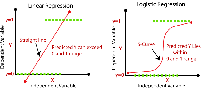
Main difference between them is how they are being used
The Linear Regression is used for solving Regression problems whereas Logistic Regression is used for solving the Classification problems.Linear Regression Logistic Regression Linear regression is used to predict the continuous dependent variable using a given set of independent variables. Logistic Regression is used to predict the categorical dependent variable using a given set of independent variables. Linear Regression is used for solving Regression problem. Logistic regression is used for solving Classification problems. In Linear regression, we predict the value of continuous variables. In logistic Regression, we predict the values of categorical variables. In linear regression, we find the best fit line, by which we can easily predict the output. In Logistic Regression, we find the S-curve by which we can classify the samples. Least square estimation method is used for estimation of accuracy. Maximum likelihood estimation method is used for estimation of accuracy. The output for Linear Regression must be a continuous value, such as price, age, etc. The output of Logistic Regression must be a Categorical value such as 0 or 1, Yes or No, etc. In Linear regression, it is required that relationship between dependent variable and independent variable must be linear. In Logistic regression, it is not required to have the linear relationship between the dependent and independent variable. In linear regression, there may be collinearity between the independent variables. In logistic regression, there should not be collinearity between the independent variable.
Theory
- Decision boundary
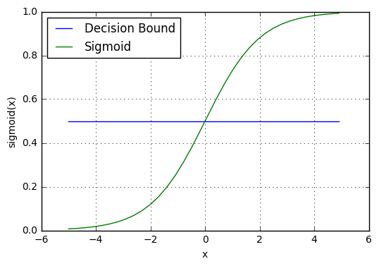
- Suppose we have a generic training set $\lbrace \left(x^{(1)}, y^{(1)}\right),\left(x^{(2)}, y^{(2)}\right), \ldots,\left(x^{(m)}, y^{(m)}\right) \rbrace$, where $𝑥(𝑚)$ is the input variable of the 𝑚-th example, while $𝑦(𝑚)$ is its output variable, ranging from 0 to 1. Finally we have the hypothesis function for logistic regression, $h_{\theta}(x)=\frac{1}{1+e^{-\theta^T x}}$.
Interpretation
The cost function used in linear regression won’t work here
- If we try to use the cost function of the linear regression in Logistic Regression $\sum^m_{i=1}(y^{(i)}-\frac{1}{1+e^{-\theta^T x}})^2$, then it would be of no use as it would end up being a non-convex function with many local minimums, in which it would be very difficult to minimize the cost value and find the global minimum.

- Logistic regression cost function
$$ cost\left(h_{\theta}(x), y\right)=\left\{\begin{array}{ll}{-\log \left(h_{\theta} (x)\right)} & {\text { if } y=1} \\ {-\log \left(1-h_{\theta}(x)\right)} & {\text { if } y=0}\end{array}\right. $$
即,$cost\left(h_{\theta}(x), y\right)=-y \log \left(h_{\theta}(x)\right)-(1-y) \log \left(1-h_{\theta}(x)\right)$
- With the optimization in place, the logistic regression cost function can be rewritten as:
$$ \begin{aligned} J(\theta) &=\frac{1}{m} \sum_{i=1}^{m} cost\left(h_{\theta}\left(x^{(i)}\right), y^{(i)}\right) \\ &=-\frac{1}{m}\left[\sum_{i=1}^{m} y^{(i)} \log \left(h_{\theta}\left(x^{(i)}\right)\right)+\left(1-y^{(i)}\right) \log \left(1-h_{\theta}\left(x^{(i)}\right)\right)\right] \end{aligned} $$
- $\frac{\partial}{\partial \theta_{j}} J(\theta)=\frac{1}{m} \sum_{i=1}^{m}\left(h_{\theta}\left(x^{(i)}\right)-y^{(i)}\right) x_{j}^{(i)}$推导过程

- $\frac{d}{d x} \sigma(x)=\sigma(x)(1-\sigma(x))$推导过程

逻辑回归的分布式实现
- 按行并行
即将样本拆分到不同的机器上去,把数据集打散(注:即“划分”,要满足不重、不漏两个条件)成 C 块,$\frac{\partial J}{\partial w}=\frac{1}{N} \sum_{k=1}^{K} \sum_{i \in C_{k}}\left(h_{\theta}\left(x^{(i)}\right)-y^{(i)}\right) \times x^{(i)}$, 然后将这 C 块分配到不同的机器上去,则分布式的计算梯度,只不过是每台机器都计算出各自的梯度,然后归并求和再求其平均。- 为什么可以这么做呢?
梯度下降公式只与上一个更新批次的$\theta$及当前样本有关
- 为什么可以这么做呢?
- 按列并行
按列并行的意思就是将同一样本的特征也分布到不同的机器中去。上面的公式为针对整个$\theta$,如果我们只是针对某个分量$\theta_{j}$,可得到对应的梯度计算公式 $ \frac{\partial J}{\partial w}=\frac{1}{N} \sum_{i=1}^{N}\left(h_{\theta_j}\left(x_{j}^{(i)}\right)-y^{(i)}\right) \times x_{j}^{(i)} $ ,即不再是乘以整个 $x_n$,而是乘以 $x_n$ 对应的分量 $x_{n,j}$,此时可以发现,梯度计算公式仅与$x_n$中的特征有关系,我们就可以将特征分布到不同的计算上,分别计算$\theta_{j}$对应的梯度,最后归并为整体的$\theta$,再按行归并到整体的梯度更新。
逻辑回归的优缺点
- Advantages of Logistic Regression
- $1.$ Logistic Regression performs well when the dataset is linearly separable.(对于非线性的数据集适应性弱)
- $2.$ Logistic regression is less prone to over-fitting but it can overfit in high dimensional datasets. You should consider Regularization (L1 and L2) techniques to avoid over-fitting in these scenarios.
- $3.$ Logistic Regression not only gives a measure of how relevant a predictor (coefficient size) is, but also its direction of association (positive or negative).
- $4.$ Logistic regression is easier to implement, interpret and very efficient to train.
- Disadvantages of Logistic Regression
- $1.$ Main limitation of Logistic Regression is the assumption of linearity between the dependent variable and the independent variables. In the real world, the data is rarely linearly separable. Most of the time data would be a jumbled mess.
- $2.$ If the number of observations are lesser than the number of features, Logistic Regression should not be used, otherwise it may lead to overfit.(当特征空间很大,性能欠佳)
- $3.$ Logistic Regression can only be used to predict discrete functions. Therefore, the dependent variable of Logistic Regression is restricted to the discrete number set. This restriction itself is problematic, as it is prohibitive to the prediction of continuous data.
- $4.$ 因为预测结果呈Z字型(或反Z字型),因此当数据集中在中间区域时,对概率的变化会很敏感,可能使得预测结果缺乏区分度。
Handling Imbalanced Classes In Logistic Regression
- Like many other learning algorithms in scikit-learn, LogisticRegression comes with a built-in method of handling imbalanced classes. If we have highly imbalanced classes and have no addressed it during preprocessing, we have the option of using the class_weight parameter to weight the classes to make certain we have a balanced mix of each class. Specifically, the balanced argument will automatically weigh classes inversely proportional to their frequency: $w_{j}=\frac{n}{k n_{j}}$, where $w_j$ is the weight to class $j$, $n$ is the number of observations, $n_j$ is the number of observations in class $j$, and $k$ is the total number of classes.
sklearn.linear_model.LogisticRegression部分参数解析
| Parameters | detail |
|---|---|
| penalty: {‘l1’, ‘l2’, ‘elasticnet’, ‘none’}, default=’l2’ | |
| dual: bool, default=False | Dual or primal formulation. Dual formulation is only implemented for l2 penalty with liblinear solver. Prefer dual=False when n_samples > n_features. |
| tolfloat: default=1e-4 | 迭代终止判断的误差范围 |
| C: float, default=1.0 | 其值等于正则化强度的倒数,为正的浮点数。数值越小表示正则化越强。 |
| fit_intercept: bool, default=True | 指定是否应该向决策函数添加常量(即偏差或截距) |
| intercept_scaling: float, default=1 | 仅仅当solver是”liblinear”时有用 |
| class_weight: dict or ‘balanced’, default=None | 调整样本不均衡问题 |
逻辑回归+牛顿法+梯度下降讲义补充


python实现(代码链接)
- 1、先尝试调用sklearn的线性回归模型训练数据,尝试以下代码,画图查看分类的结果
- 2、用梯度下降法将相同的数据分类,画图和sklearn的结果相比较
- 3、用牛顿法实现结果,画图和sklearn的结果相比较,并比较牛顿法和梯度下降法迭代收敛的次数