Linear Regression

线性回归的原理

线性回归的一般形式
LinearRegression fits a linear model with coefficients $w = (w1, …, wp)$ to minimize the residual sum of squares between the observed targets in the dataset, and the targets predicted by the linear approximation.
Why do we use the Mean-Squared Loss(MSE)?

线性回归损失函数、代价函数、目标函数

Objective function, cost function, loss function: are they the same thing?

线性回归的优化方法

Gradient Descent

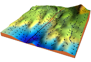
Consider the 3-dimensional graph below in the context of a cost function. Our goal is to move from the mountain in the top right corner (high cost) to the dark blue sea in the bottom left (low cost). The arrows represent the direction of steepest descent (negative gradient) from any given point–the direction that decreases the cost function as quickly as possible.

What is the objective of Gradient Descent?
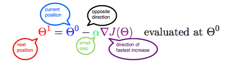
Gradient, in plain terms means slope or slant of a surface. So gradient descent literally means descending a slope to reach the lowest point on that surface.
Gradient descent is an iterative algorithm, that starts from a random point on a function and travels down its slope in steps until it reaches the lowest point of that function.
The Point of GD
Minimizing any cost function means finding the deepest valley in that function. Keep in mind that, the cost function is used to monitor the error in predictions of an ML model. So, the whole point of GD is to minimize the cost function.

Learning rate
The size of these steps is called the learning rate. With a high learning rate we can cover more ground each step, but we risk overshooting the lowest point since the slope of the hill is constantly changing. With a very low learning rate, we can confidently move in the direction of the negative gradient since we are recalculating it so frequently. A low learning rate is more precise, but calculating the gradient is time-consuming, so it will take us a very long time to get to the bottom.
Now let’s run gradient descent using our new cost function. There are two parameters in our cost function we can control: m (weight) and b (bias). Since we need to consider the impact each one has on the final prediction, we need to use partial derivatives. We calculate the partial derivatives of the cost function with respect to each parameter and store the results in a gradient.
- Given the cost function:
  $$ f(m,b)=\frac{1}{N}\sum (y_i-(mx_i+b))^2 $$
- The gradient can be calculated as:
$$ {f}'(m,b)=\begin{bmatrix} \frac{df}{dm}\\ \frac{df}{db} \end{bmatrix}=\begin{bmatrix} \frac{1}{N}\sum -2x_i(y_i-(mx_i+b))\\ \frac{1}{N}\sum -2(y_i-(mx_i+b)) \end{bmatrix} $$
```
    
  def update_weights(m, b, X, Y, learning_rate):
      m_deriv = 0
      b_deriv = 0
      N = len(X)
      for i in range(N):
          m_deriv += -2*X[i] * (Y[i] - (m*X[i] + b))
          b_deriv += -2*(Y[i] - (m*X[i] + b))

      //We subtract because the derivatives point in direction of steepest ascent
      m -= (m_deriv / float(N)) * learning_rate
      b -= (b_deriv / float(N)) * learning_rate

  return m, b
```
开销分析
Suppose we have 10,000 data points and 10 features. The sum of squared residuals consists of as many terms as there are data points, so 10000 terms in our case. We need to compute the derivative of this function with respect to each of the features, so in effect we will be doing 10000 * 10 = 100,000 computations per iteration. It is common to take 1000 iterations, in effect we have 100,000 * 1000 = 100000000 computations to complete the algorithm. That is pretty much an overhead and hence gradient descent is slow on huge data.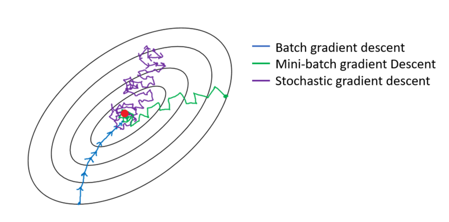

Stochastic Gradient Descent (SGD)

Where can we potentially induce randomness in our gradient descent algorithm??
Yes, you might have guessed it right !! It is while selecting data points at each step to calculate the derivatives. SGD randomly picks one data point from the whole data set at each iteration to reduce the computations enormously.
Mini-batch gradient descent
It is also common to sample a small number of data points instead of just one point at each step and that is called “mini-batch” gradient descent. Mini-batch tries to strike a balance between the goodness of gradient descent and speed of SGD.
梯度下降法的缺陷：如果函数为非凸函数，有可能找到的并非全局最优值，而是局部最优值。

最小二乘法矩阵求解

The Least Squares Regression Line
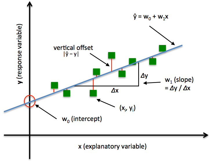
The Least Squares Regression Line is the line that makes the vertical distance from the data points to the regression line as small as possible. It’s called a “least squares” because the best line of fit is one that minimizes the variance (the sum of squares of the errors).

Goal: to find the line (or hyperplane) that minimizes the vertical offsets
以估计房价为例，假设真实世界里房子的面积 x与房价 y 的关系是线性关系，且真实世界存在无法估计的误差 $\epsilon$，也就是 $y=w_0+w_1 x+\epsilon $，最小二乘法就是要找到使误差 $\epsilon$ 的平方和最小的 $w_0$，$w_1$即可。

$$ y=Xw+\epsilon $$

$$ \underset{w}{min} \ \epsilon^T \epsilon $$
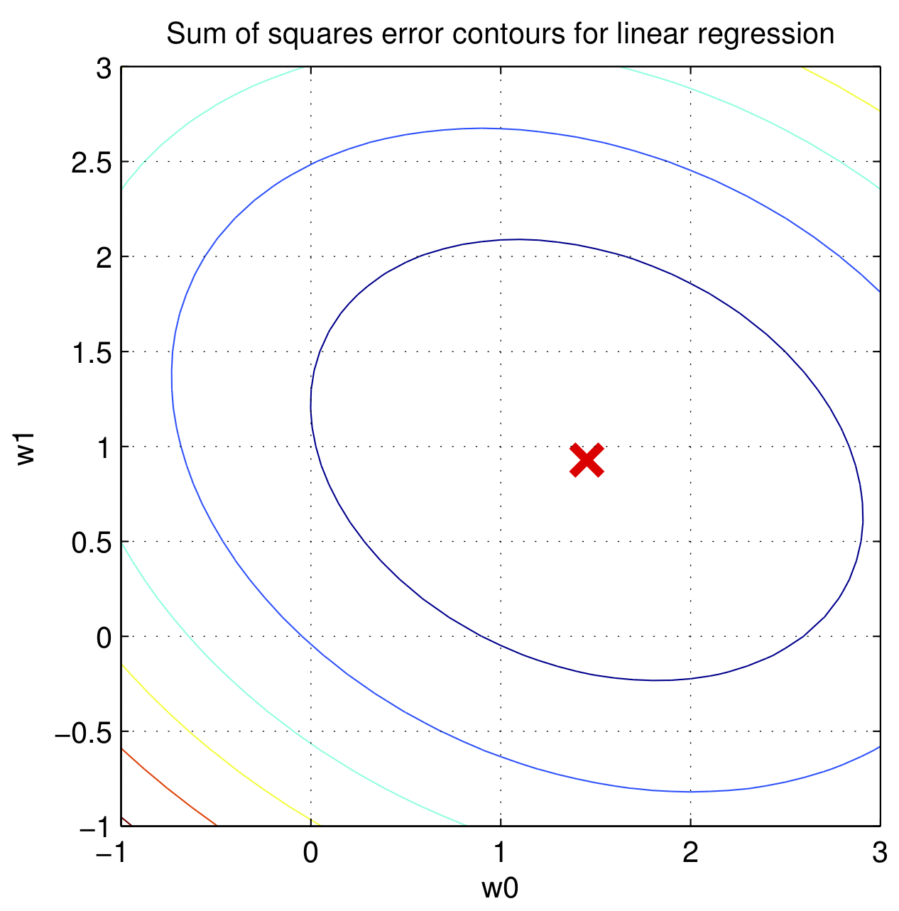
$\epsilon^T \epsilon$的图像像一个碗
- 如下图所示，这意味着存在一个全局最低点，这样的函数叫做凸函数，可以使用梯度下降法来得到全局最低点对应的的 w ，这里不再赘述，只讲用微积分直接求解（最小二乘法）。
$$ \nabla_w\epsilon^T \epsilon = 2X^TXw-2X^Ty $$
- 当 $\nabla_w\epsilon^T \epsilon=0$时，得到位置$\widehat{w} = (X^TX)^{-1}X^Ty$

OLS与GD的关联

Simple Linear Regression — OLS vs Mini-batch Gradient Descent (Python)

Two approaches to fit a linear regression model are:
- Ordinary Least Squares (OLS) (an analytical method)
  1.Normal Equations (closed-form solution):
  2.OLS is easy and fast if the data is not big.
  3.The closed-form solution may (should) be preferred for “smaller” datasets – if computing (a “costly”) matrix inverse is not a concern. For very large datasets, or datasets where the inverse of $X^TX$ may not exist (the matrix is non-invertible or singular, e.g., in case of perfect multicollinearity), the GD or SGD approaches are to be preferred.
- Gradient Descent (GD) (a numerical method)
  GD is beneficial when the data is big and memory is limited.

牛顿法

Suppose that we want to approximate the solution to $f(x)=0$ and $0=f\left(x_{0}\right)+f^{\prime}\left(x_{0}\right)\left(x_{1}-x_{0}\right)$, so we get $x_{1}=x_{0}-\frac{f\left(x_{0}\right)}{f^{\prime}\left(x_{0}\right)}$.
So, we can find the new approximation provided the derivative isn’t zero at the original approximation. If $x_{n}$ is an approximation a solution of $f(x)=0$ and if $f^{\prime}\left(x_{n}\right) \neq 0$ the next approximation is given by, $x_{n+1}=x_{n}-\frac{f\left(x_{n}\right)}{f^{\prime}\left(x_{n}\right)}$.
Taylor series – approximating a function
Taylor series is an approximation of a function using series expansion. Taylor series of function $f(x)$ around axis $x=a$ can be written below. $f(x) \approx f(a)+\frac{f^{\prime}(a)}{1 !}(x-a)+\frac{f^{\prime \prime}(a)}{2 !}(x-a)^{2}+\frac{f^{\prime \prime \prime}(a)}{3 !}(x-a)^{3}+\ldots$.
Newton’s method for optimization
After we know how Newton’s method works for finding root, and Taylor series for approximating a function, we will try to expand our Newton’s method for optimization, finding the minimal value of a function.
- Newton’s method for finding root, it uses first order method.
- Newton’s method for optimization, it use second order method.
  - Second approximation of f(x) around axis x=a is as follows.
    
    Then, in order to get the minimal value location of approximation above, we take the first differential, and make it equal to zero. Here we go.
    
    Voila! We just derived our Newton’s method for optimization. To find minimal value of our cost function in machine learning, we can iterate using this equation

Why is Newton’s method not widely used in machine learning?

拟牛顿法

在牛顿法的迭代中，需要计算 Hessian 矩阵的逆矩阵，计算过程较复杂，考虑采用一个 n 阶矩阵 $G_{k}=G\left(x_{k}\right)$ 近似替代 $H_{k}^{-1}=H^{-1}\left(x_{k}\right)$，这就是拟牛顿法的基本思想。
拟牛顿条件
$$ \begin{aligned} & \nabla f\left(x_{k+1}\right)=\nabla f\left(x_{k}\right)+H_{k}\left(x_{k+1}-x_{k}\right) \\ \Rightarrow & H_{k}^{-1} \cdot\left(\nabla f\left(x_{k+1}\right)-\nabla f\left(x_{k}\right)\right)=x_{k+1}-x_{k} \end{aligned} $$
- 常用的求解拟牛顿的算法有DFP算法、BFGS算法、Broyden类算法。

python实现(代码链接)

1、首先尝试调用sklearn的线性回归函数进行训练
2、用最小二乘法的矩阵求解法训练数据
3、梯度下降法

线性回归

线性回归的原理

线性回归损失函数、代价函数、目标函数

线性回归的优化方法

Gradient Descent

Stochastic Gradient Descent (SGD)

Mini-batch gradient descent

最小二乘法矩阵求解

OLS与GD的关联

牛顿法

拟牛顿法

python实现(代码链接)

CATALOG

FEATURED TAGS